Finding damaged strands on power cables: Strand geometry and a frozen foundation model, tested on cables their developers never saw
Inspection robots film overhead power cables, and a person then has to find the few frames that show damage. CableInspect-AD is the public benchmark for doing this from healthy footage alone: each fold gives 100 healthy frames of one cable to train on, and the best published method scores 0.86 image AUROC. Our method aligns the cable in every frame and adds five scores: two reconstruction models, two models of the strands’ helical geometry, and a detector on a frozen DINOv3 model trained on defects drawn in code. With each cable held out from the AI agents that developed the recipe for it, it scores 0.951. That is the same as on the cables it was developed on (0.952), and above all thirteen recent methods we re-ran and tuned the same way (best 0.931). Most of the gain comes from the alignment, which lifts Dinomaly alone from 0.891 to 0.931. The fusion adds 0.019 over a Dinomaly frozen under the same conditions, mostly on light spaced strands. The operating point is not solved: a threshold set from healthy training frames to flag 5% of healthy frames flags 10% on unseen cables.
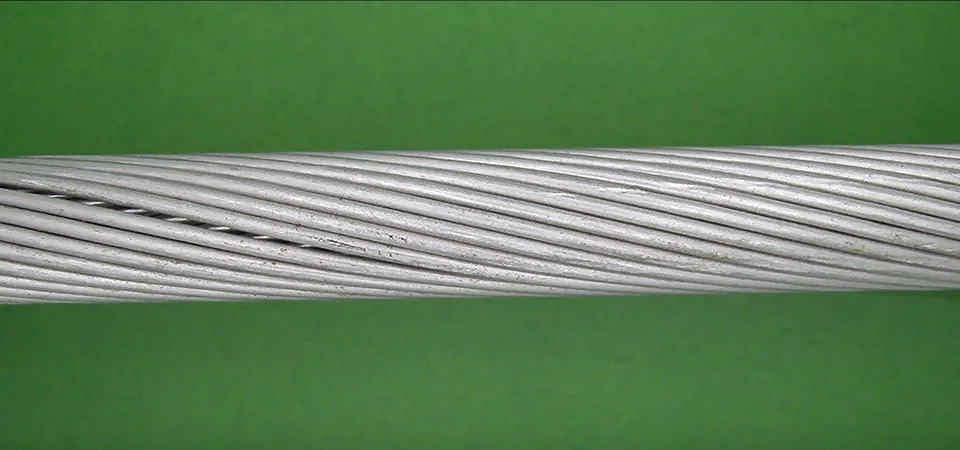 A Raw frame
 B Aligned view
 C Detection map
Image-level AUROC, higher is better. Over 116 folds the protocol averages each cable’s folds and then the three cables, as in the dataset paper; where a ± is given, it is the standard deviation of those three per-cable values, so it describes the spread between cables, not a confidence interval. The 0.86 is a 19-billion-parameter vision-language model used zero-shot on the raw frame, a different setting from ours; the like-for-like comparison is with re-run methods on the same view and folds. No defect labels are used at training time. Cables 1 and 2 were our development cables, so the 0.952 includes them. The 0.951 holds out each cable from the team that developed the recipe for it, and the recipes differ in some settings (section 5). Every number is in Appendix C.
1The dataset
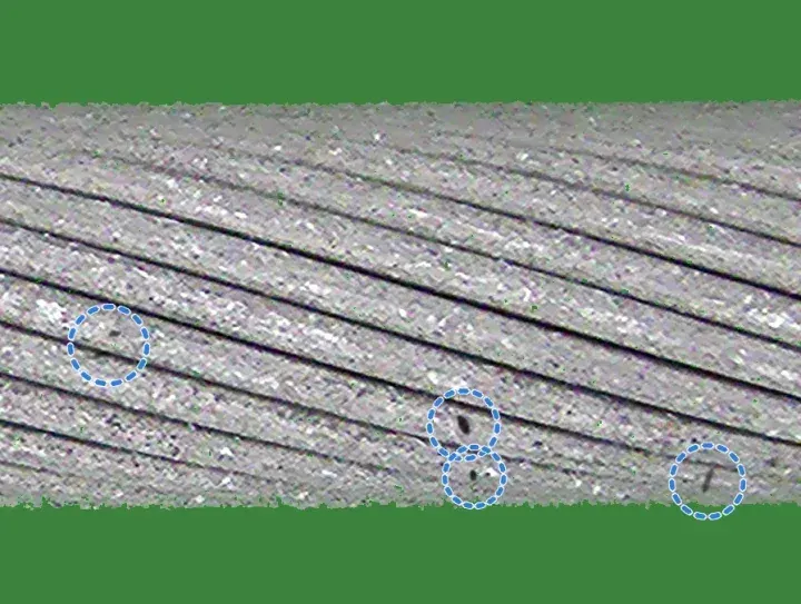
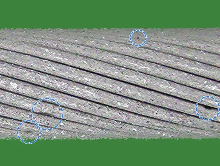
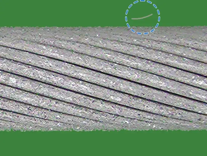
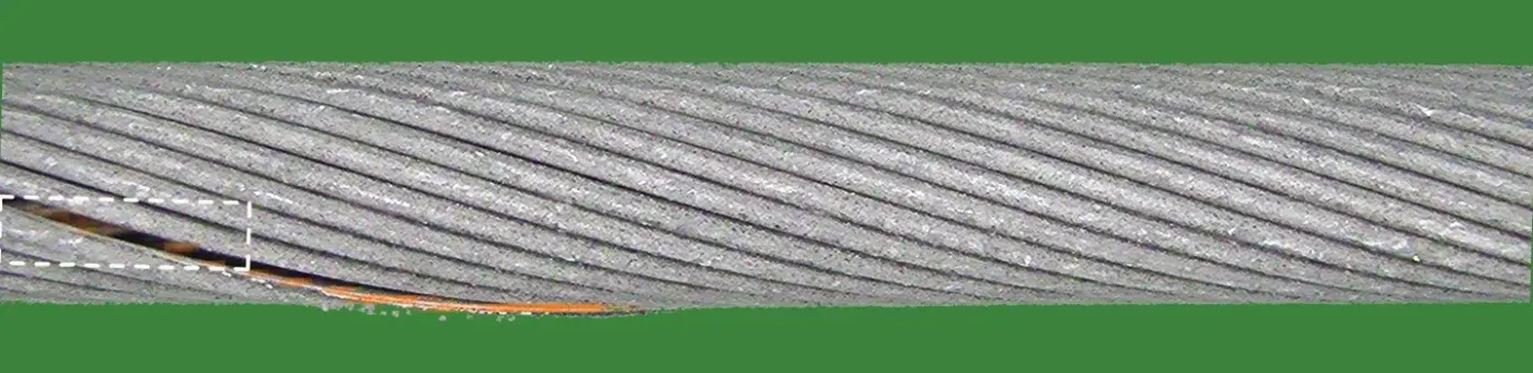
Overhead conductors are made of helically wound aluminium strands. The damage to be found is broken, bent, spaced or welded strands, crushing, deposits or scratches. On a real line damage is rare, and it ranges from a thick weld bead to a single strand sitting a millimetre further from its neighbour. The same stretch of cable also looks different on every pass of the camera.
CableInspect-AD films three real cables in a lab rig against a green screen.1 Frames are 1920×1080, and each side of a cable is filmed in three passes. Experts from Hydro-Québec labelled seven kinds of damage with boxes, each by grade. The released labels hold 4,798 frames: 2,054, 1,567 and 1,177 for cables 1, 2 and 3. Of these, 2,639 show a defect and 2,159 are healthy. The most common kind, light spaced strands, appears in about 107 test frames per fold.
2Prior work
Methods evaluated on CableInspect-AD
The dataset paper evaluates few-shot anomaly detectors and vision-language models under one protocol (section 4).1 Its Enhanced-PatchCore, a PatchCore variant,2 scores 0.78 AUROC. Its best AUROC, 0.86, comes from CogVLM2-19B used zero-shot, which flags only 4% of healthy frames but finds few defects (F1 0.66). One later method is specific to cables: INP-Former with a multi-granularity aggregation module and a voting step.5 Only its abstract is accessible and it gives no absolute numbers, so we cite it and do not compare.
Limitations of published evaluations
- A resize without anti-aliasing. The reference code shrinks the frame to 224×224 with a bilinear resize that samples without anti-aliasing. Doing the same reproduces the published PatchCore row; an anti-aliased resize alone is worth +0.03 AUROC (section 5).
- Thresholds on frames the model trained on. The protocol fits the threshold on training-frame scores, but a trained network scores its own training frames near zero, so its threshold ends up too low; SuperSimpleNet flagged every healthy dev frame this way. Under this rule, F1 and FPR of trained methods are measured at thresholds that flag too many healthy frames.
- No test on a cable kept out of development. Every published method, and every method we re-ran, was designed with all three cables in view. Only a cable kept out of development tests a method cleanly. In three sealed rebuilds of an earlier version of our method, the margin over Dinomaly fell from +0.010–0.017 on the development folds to +0.003–0.009 on the held-out cable (Appendix A). The final method kept its margin when each cable was held out: +0.015 to +0.024 (section 5).
Approaches to few-shot anomaly detection
Recent methods fall into three families. Memory banks (PatchCore, AnomalyDINO, SuperADD) store patch features of the training images and score a test patch by its distance to the nearest stored one. Reconstruction methods (Dinomaly, Dinomaly2, INP-Former) train a decoder to rebuild frozen foundation-model features from healthy images; it rebuilds healthy patches well and anomalies poorly. Synthetic-anomaly methods (GLASS, SuperSimpleNet) paste or simulate defects onto healthy images and train a classifier. We re-ran thirteen of these, each tuned on the same dev folds, once on the whole frame and once on our aligned view (section 3). On the aligned view the best is Dinomaly, at 0.931.4
3Approach
We designed the method from the errors of an earlier fusion of Dinomaly and a first strand model. On the development cables, about half of its defect-side ranking errors were light spaced strands, and its false alarms were healthy cable with scuffs, or with loose fibres on the background (section 6). The method therefore adds two channels that measure the strands’ geometry, and a detector trained with scuffs and fibres drawn as healthy. Each frame is scored on its own, and each per-fold model sees only that fold’s 100 healthy frames and data made from them.
Aligned view
The three camera passes over a cable side differ, so 100 healthy frames cover healthy cable unevenly. Between passes the cable sits up to about 130 px higher or lower in the frame and at a different tilt, the exposure changes, and parts of the rig come into view. A healthy frame from a pass that is under-represented in the training frames scores as anomalous for every method we ran.
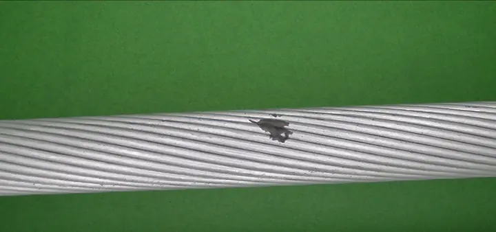
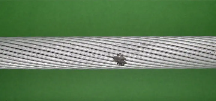
The aligned view maps each 1920×1080 frame to a strip in which the cable is horizontal, of fixed thickness and at fixed exposure. It is computed from that frame alone, without labels or other frames, in six steps.
- Background. A pixel is green screen when its green value exceeds both other channels by a factor of 1.12 and by at least 20 grey levels: G > 1.12·max(R, B) and G − max(R, B) > 20. The absolute margin keeps dark grooves between strands, which are only slightly green, in the foreground.
- Pose. On a 4× area-downsampled copy of the frame, the cable is the largest 8-connected foreground component. For every image column x that contains it we take the cable’s vertical centre of mass c(x) and its height in pixels t(x). A line c(x) = ax + b is fitted by least squares and refitted twice on the 80% of columns with the smallest residuals, which makes it robust to protruding strands. The axis angle is θ = arctan a, the thickness T = 4·medianx t(x)·cos θ in frame pixels, and the centre is the fitted axis at the middle column. Frames without foreground, or with T outside 150 to 800 px, are rejected; none of the 4,798 frames is.
- Warp. The frame is rotated by θ about the cable centre and scaled isotropically by s = 224/T, so the cable is 224 px thick and its axis lies on the middle row of a 448 px strip, with half a diameter of margin above and below for strands that stick out. The strip is round(1920·s) wide, 1,109 to 1,558 px (median 1,453), so the cable is always downsampled (s ≈ 0.58 to 0.81). A Gaussian prefilter with σ = 0.5/s precedes bilinear resampling; regions outside the frame are filled with a constant green.
- Exposure. A single gain k = clip(160/g, 0.6, 1.6) multiplies all channels, where g is the median, over the cable’s pixels, of the mean of the three colour channels.
- Background replacement. Every background pixel is set to one flat green (RGB 60, 130, 60). Of the foreground components, the cable is always kept, and any other component of at least 40 px is kept unless it touches the top or bottom edge of the strip: loose strands floating near the cable stay, rig equipment entering from the border goes.
- Tiles. Four 448×448 tiles are cut with left edges evenly spaced from 0 to W − 448, so neighbouring tiles overlap (by about 113 px at the median width); there is no padding or resizing.
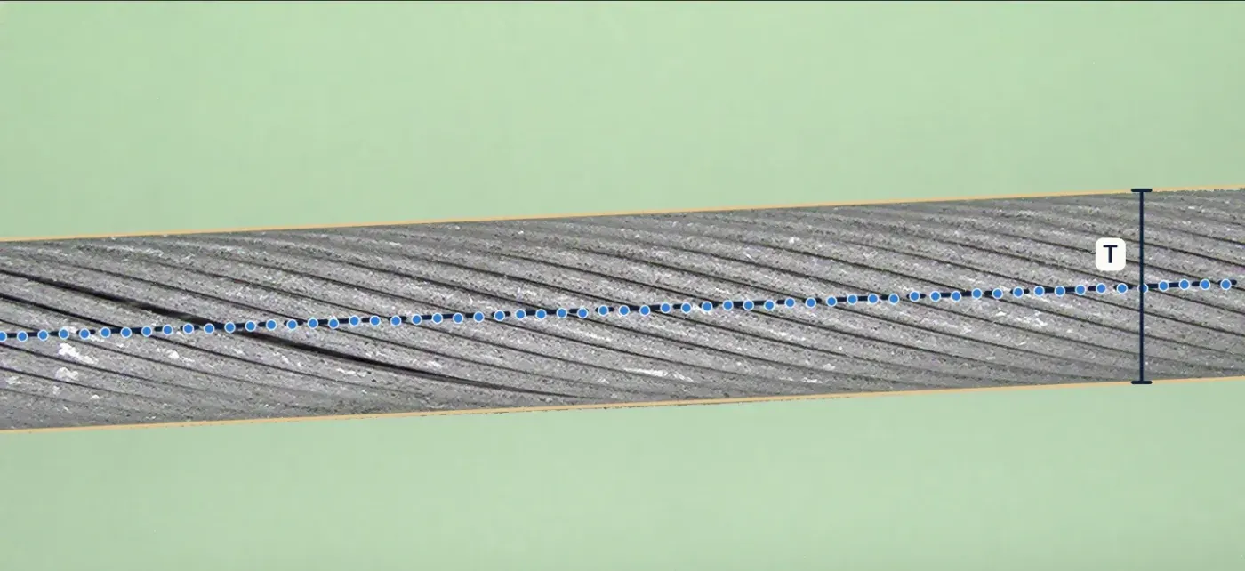 A Raw frame, pose
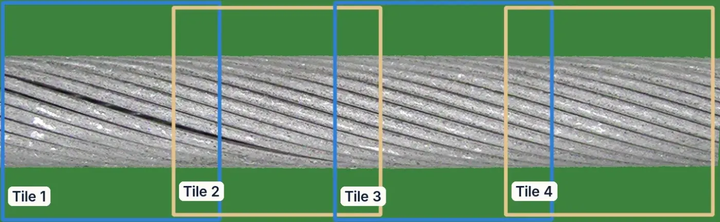 B Aligned view, 4 tiles
Two higher-resolution versions are built from the same pose and exposure. The 1.9× view crops rows 106 to 342 of the strip (the cable plus about 6 px of its outline), upsamples them bicubically by 448/236 ≈ 1.9 and cuts seven evenly spaced 448 px tiles. The detector strip re-renders the raw frame with the cable 448 px thick in an 896 px tall strip, using bicubic interpolation, so the cable is sampled at 1.15 to 1.6 times its resolution in the frame.
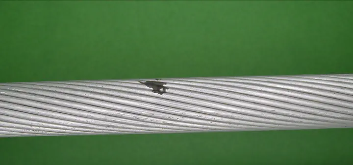



Reconstruction channels
Two Dinomaly models4 are trained per fold on all 100 healthy training frames, with anomalib 2.7 and its default architecture: a frozen ViT-B/14 DINOv2 encoder with registers,3 blocks 2 to 9 fused into two groups, a bottleneck MLP (dropout 0.2) and eight linear-attention decoder blocks, trained to reconstruct the encoder’s features with a cosine loss that mines hard tokens, with StableAdamW (learning rate 2·10⁻³) for 1,000 steps at batch 16 in bf16.
- Anomaly map. For each group, one minus the cosine similarity between encoder and decoder features per token, averaged over the two groups, upsampled, resized to 256×256 and smoothed with a Gaussian (σ = 4). A tile’s score is the mean of its highest 1% of pixels, and a frame’s score is the maximum over its tiles.
- Inputs. The 1× channel reads the four 448 px tiles of the aligned strip (32×32 tokens each). The 1.9× channel reads the seven tiles of the 1.9× view, where a token covers about 7 strip pixels instead of 14.
- Learning-rate schedule. anomalib 2.7 returns Dinomaly’s warm-up-and-cosine scheduler without a per-step interval, so it advances once per epoch. In these two channels that was not corrected: with 25 and 43 steps per epoch, the schedule stays in its 100-iteration warm-up for the whole run, so the learning rate rises linearly to about 8·10⁻⁴ and 5·10⁻⁴ and never decays. The settings were chosen on the development folds with this behaviour. The re-run baselines of section 2 use the per-step fix (Appendix B).
Strand lattice
The cable’s outer layer is a lattice of strands separated by dark grooves, and a healthy strand looks like its neighbours seen from the same angle. The lattice channel compares each strand with exactly those neighbours. It needs no learning beyond a normal model of its residuals, and it is computed on the aligned strip in four steps.
- Unwrapping. The cable band (rows whose foreground share exceeds 0.5, with centre c and radius R) is resampled onto 258 rows spaced uniformly in viewing angle φ ∈ [−1.15, 1.15] rad, reading source row c + R sin φ with bilinear interpolation; columns stay axial positions x. Slow illumination is removed by subtracting a Gaussian blur (σ = 12 px), which leaves a detail image D.
- Lay and period. One lay slope s (rows per pixel) is estimated per frame by maximising the correlation of D with itself under a column offset (coarse: 16 px offset, ±7 rows; fine: 96 px, ±6 rows around the coarse value, parabolic peak). The axial period P, the shift that maps each strand onto its neighbour, is the peak of the row-summed, overlap-normalised autocorrelation along the cable for lags of 60 to 180 px. Shearing D by r′ = r − s x makes strands horizontal, with expected groove spacing Δ = sP.
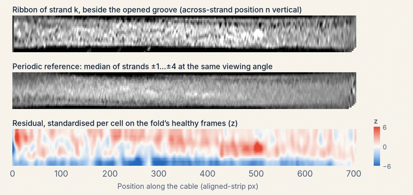
- Grooves and ribbons. Grooves are local minima, at least 0.6Δ apart and below the median, of profiles averaged over 48 px column blocks every 16 px (smoothed with σ = 1.5 rows). They are linked left to right into tracks (largest step 0.3Δ, at most 3 blocks missing, at least 5 detections), smoothed with a 5-block running median and interpolated to every column, so a lay that drifts along the frame is followed rather than assumed straight. Strand k is then resampled as a ribbon between grooves k and k+1: 24 rows at normalised across-strand positions n = (i+½)/24, at every column, each sample keeping its viewing angle.
- References and residuals. The periodic reference of ribbon k at column x is the median, over j = ±1…±4, of ribbon k−j at column x + round(jP) and the same n: the strand j places along the lattice, seen at the same angle. The residual (ribbon − reference, blurred with σ = 3) is standardised per cell, where a cell is a 16-row viewing-angle band (about 8°) and an across-strand position, using the median and 1.4826·MAD of all training-frame residuals in that cell (spread floored at half the median cell spread), and clipped to ±6. A self-reference residual is computed the same way on the whole unwrapped image, without ribbons: D minus the median of 8 copies shifted by ±1…±4 periods along the cable, each registered by a smooth vertical shift field of at most 4 rows.
 A Detail image D
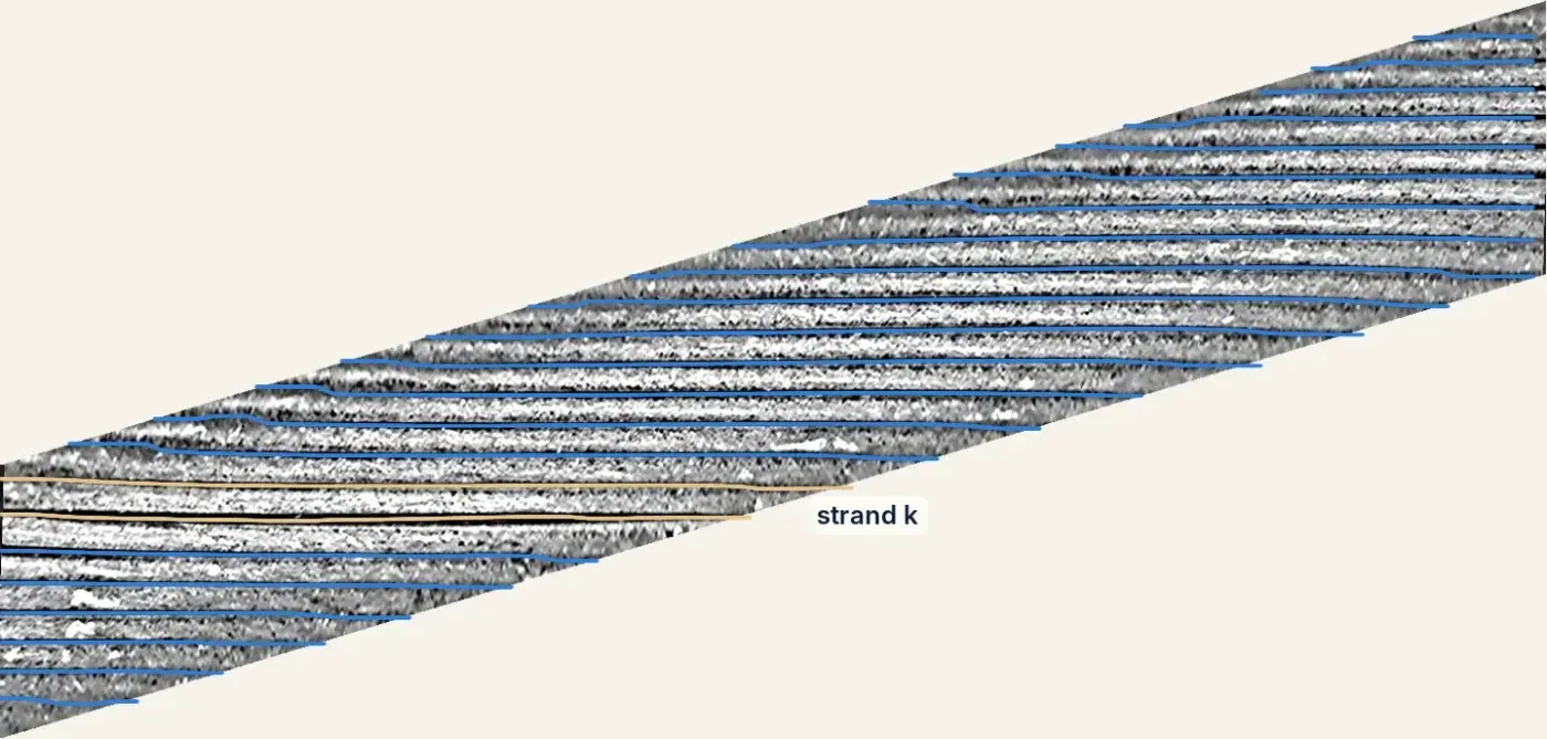 B Sheared, grooves tracked
The frame is summarised by 12 features. Eight come from the periodic residual: for each sign, the largest scan statistic Σz/√n over windows of 16 to 256 px along any ribbon row (at least 75% covered), separately for the three outer rows on each side and the six central rows, and the maximum and 0.999 quantile of z. Four come from the self-reference residual: the 0.999 quantiles of the residual averaged along the lay over 101 px (signed and absolute), of the residual blurred with σ = 4 px, and its RMS. Each feature is standardised with the median and 1.4826·MAD over the fold’s 100 training frames and clipped to [−5, 25]; the lattice score is the largest of the twelve. Training-frame scores are cross-fitted: the normal model is refitted five times, each time leaving out a block of 20 training frames, which are then scored with it.
Helical test
A spaced strand is a strand displaced from its place in the helix, which shows as a groove that is a little too wide, or a strand that is a little too wide, over some length. The helical channel models the outer layer explicitly and tests each groove for such a sustained shift.
- Geometry. The cable’s edges are located to sub-pixel accuracy, at the half-contrast crossing of a green-excess map (G − max(R, B), blurred with σ = 1 px), and each edge is fitted by a quadratic in the column with trimmed least squares (four refits, each keeping the best 80% of columns). This gives the axis, its tilt and the apparent radius rs. The cable is modelled as a cylinder seen by a pinhole camera at distance d cable radii from the axis: a surface point at axial position u and azimuth φ appears shifted sideways by Rf·(d−1) sin φ / (d − cos φ), with Rf = rs√((d+1)/(d−1)). The frame is resampled bicubically onto a (φ, u) grid with one front-line pixel of arc per row, for |φ| ≤ 1.15 rad, and slow illumination is removed (Gaussian, σ = 14 px).
- The helix. In this unwrapped image the grooves between outer strands are parallel lines, row = φ0 + m u + jΔ for integer j, with lay angle α = arctan m, circumferential spacing Δ and phase φ0. These are estimated from the frame alone by maximising the normalised coherence between the image and the matching plane wave, starting from the peak of its 2D power spectrum (25 ≤ Δ ≤ 110 rows, |m| ≤ 0.8) and refined with Nelder–Mead. The camera distance is the value in d ∈ {8, 12, 20, 40, ∞} that gives the most coherent lattice.
- Measurements. Every 4 px along each groove, a cross-groove profile spanning ±Δ/2 is averaged over 9 positions ±8 px along the groove. From it we take the sub-pixel groove bottom (the minimum within 0.3Δ of the lattice line, refined by a parabola), the full width at half depth, and a contrast-invariant position and stretch from correlating the profile with the frame’s median groove profile over shifts and stretches of 0.6 to 1.8.
- Features. Five dimensionless features per groove sample: the groove’s position after removing a robust quadratic trend in (u, φ), the half-depth width, the gap to the next groove minus its frame median (the apparent width of the strand below), and the template-based versions of the last two, each divided by Δ. Three sums, gapj−1 + gapj + widthj, gapj + widthj and its template analogue, encode the widening of both strands next to a displaced one.
- Normal model, fitted per fold on its training frames only. Each feature is standardised with the median and 1.4826·MAD of the training samples in its viewing-angle bin (12 bins of 0.2 rad, spread floored at a quarter of the feature’s median spread); the median of the three neighbouring grooves on either side is subtracted, which removes effects common to the whole stretch; the result is whitened along each groove with an AR(2) model fitted by Yule–Walker; and the innovations are mapped to a standard normal through their empirical training quantiles, separately for three bands of |φ|. The three sums are formed from these and rescaled by their training spread.
- Sequential test. On each of the 8 channels and for both signs, Page’s CUSUM, St = max(0, St−1 + δεt − δ²/2), runs along every groove in both directions for δ ∈ {0.25, 0.5, 1, 2}; missing samples add nothing. Its maximum is the log-likelihood ratio of a mean shift of δ over the best-placed segment, so a small widening over a long stretch can score as high as a large one over a short stretch. A channel’s frame statistic is its maximum over grooves and positions. Two silhouette statistics are added: the largest smoothed amount of cable outside and missing inside the fitted edges.
- Calibration. Each of the 66 statistics is turned into −log10 p against the same statistic on the fold’s healthy training frames, extended beyond the largest of them by an exponential tail fitted on their top 20%, and the frame score is the largest calibrated statistic. The training-frame statistics are cross-fitted by leaving one camera pass out at a time, so the reference includes the change of pose between passes that test frames undergo.
 A Unwrapped (φ, u), fitted lattice
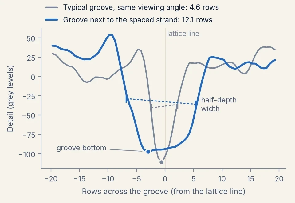
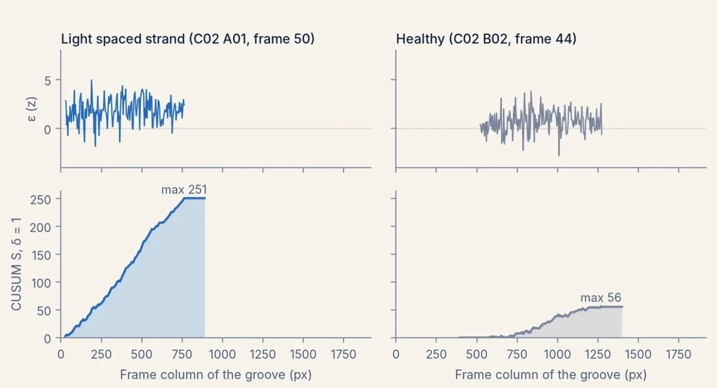
On their own the lattice and helical channels reach 0.76 to 0.88 AUROC over all kinds of damage. They are added because they detect light spaced strands that reconstruction misses, and rarely fire on healthy frames.
Learned detector
The detector is a small segmentation head on a frozen foundation model, trained per fold on that fold’s healthy frames with defects drawn onto them.
- Backbone and head. DINOv3 ViT-L/166 (LVD-1689M weights), frozen and kept in bf16, reads the detector strip (cable 448 px thick). The token maps of blocks 6, 12, 18 and 24 are concatenated (4,096 channels at stride 16) and passed through a 1×1 convolution to 256 channels, a 3×3 convolution (each followed by GroupNorm and GELU) and a 1×1 convolution, giving one defect logit per 16×16 px token.
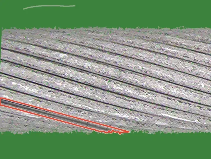
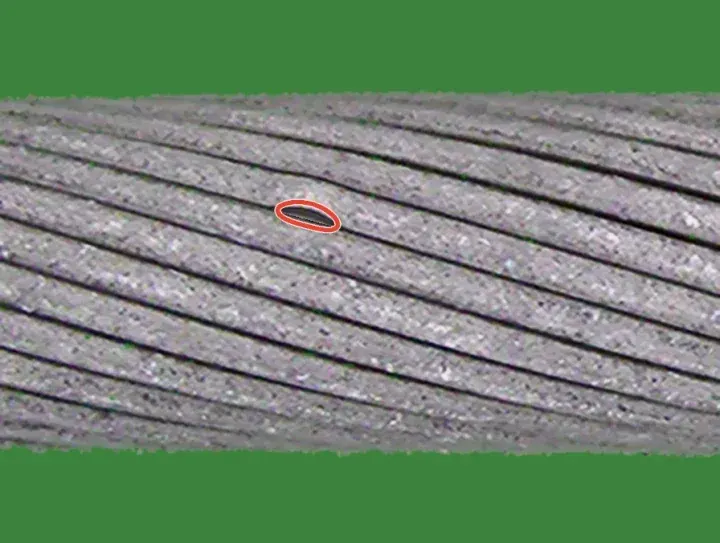
- Training data. Of the 100 training frames, positions 2, 7, …, 97 are held out and the head is fitted on the other 80, on 12,000 crops of 896×896 px (1,500 steps of 8). Every crop gets healthy variation: contrast, brightness, white balance, blur and noise, plus marks that stay labelled healthy, namely wear specks, short dark groove dashes, faint scuffs, small neutral dark pits (probability 0.5) and loose fibres lying on the background near the cable (probability 0.15). With probability 0.65 a crop then receives one to three visible synthetic defects. Families are drawn with probabilities 0.23 spaced strand, 0.13 scratch, 0.13 deposit, 0.11 speckled deposit, 0.09 cut strand, 0.07 crush mark, 0.07 rotated paste of the same cable, 0.06 bent strand, 0.05 extracted strand and 0.05 weld. Spaced and bent strands are made by warping the pixels on one side of a groove across the lay, over 120 to 1,800 px of strip for spaced and 60 to 440 px for bent strands, revealing a darkened inner layer; scratches mostly follow the lay and sit on strand crowns. 30% of crops touch a strip end, and in half of those the defect is placed within 0.45 cable thicknesses of it, so it runs out of view. A token is positive when the soft defect mask reaches 0.3 inside it.
- Loss and optimisation. Token-wise binary cross-entropy plus a hard-negative term, the mean softplus of the 16 highest healthy-token logits in each crop, with weight 1. Only the head is trained: AdamW (learning rate 5·10⁻⁴, weight decay 0.05), 100 warm-up steps and cosine decay, bf16, gradient clipping at 1. An exponential moving average of the head (decay 0.998) is used for scoring.
- Frame score. The strip is scored in 896 px windows at stride 448, overlapping logits are averaged, and the frame score is the mean of its 30 highest token logits, chosen on the development folds from six aggregations.
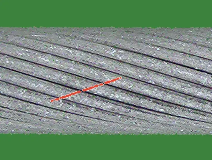
 Spaced, at strip end
 Bent strand
 Crown scratch
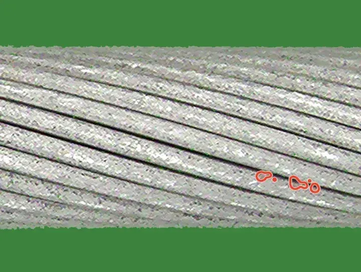 Speckled deposit
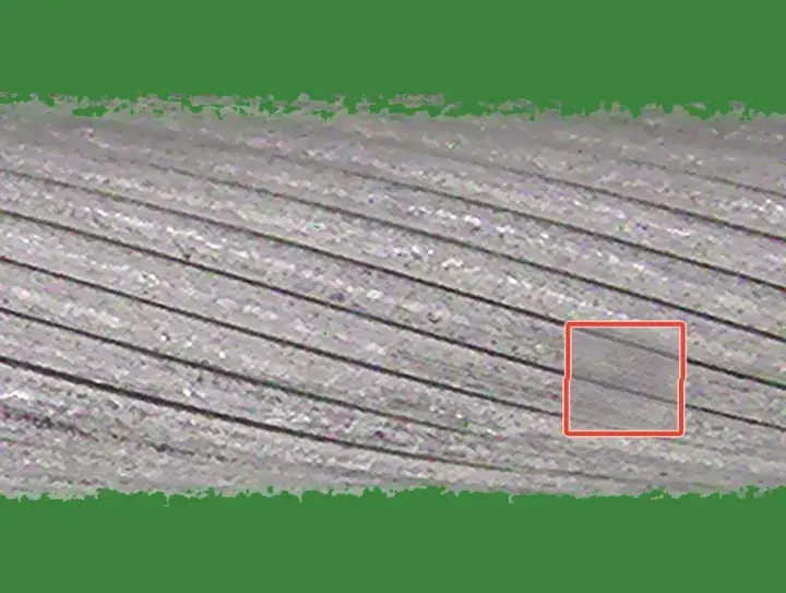 Crush
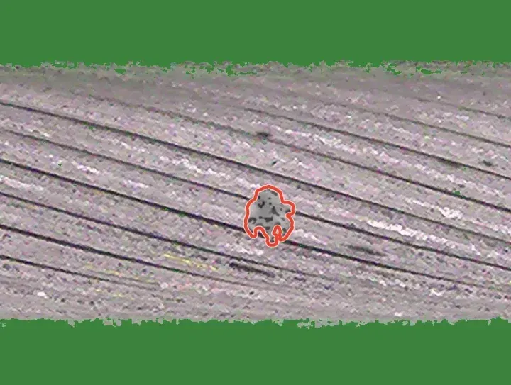 Weld blob
 Pits
 Groove dashes
 Loose fibre
 C1 Light spaced strand at the frame edge · z = 21.0
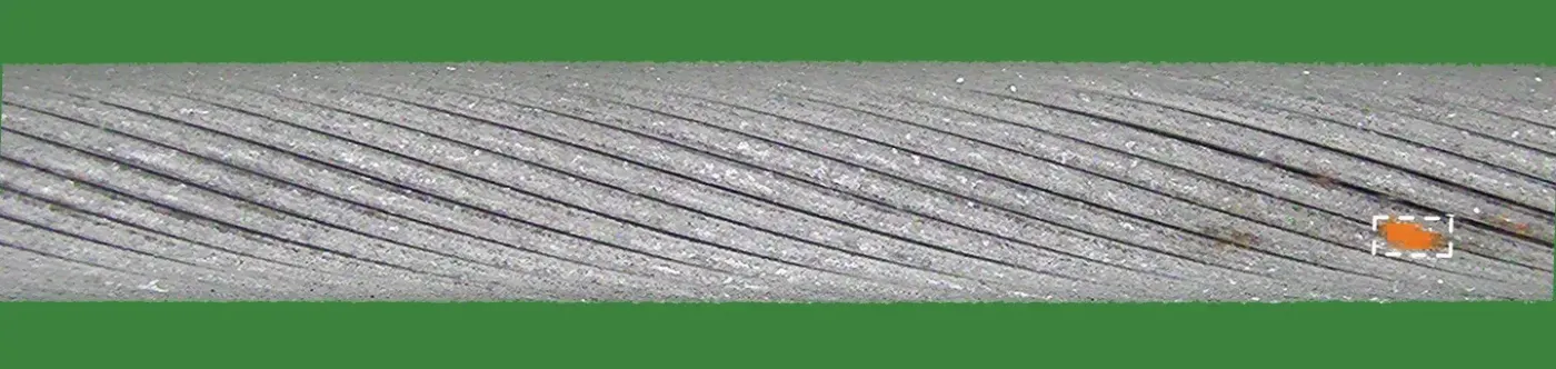 C2 Light deposit · z = 19.7
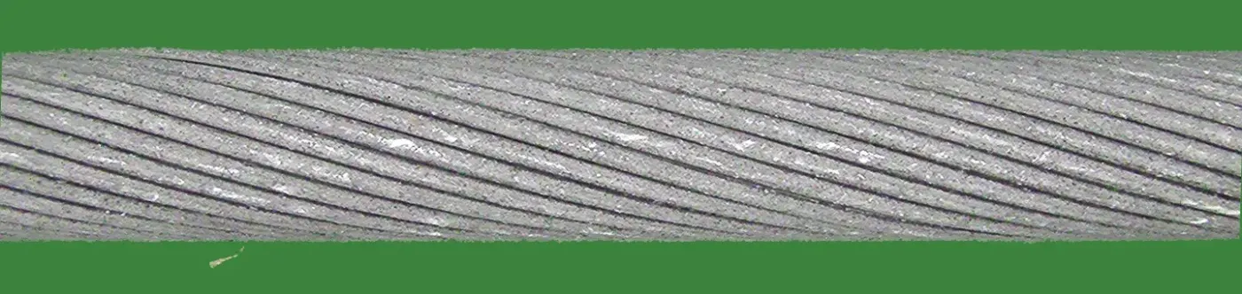 C3 Healthy, loose fibre below the cable · z = −1.6

We tested two alternatives. With the backbone fine-tuned, the detector alone scored 0.935 and 0.842 on the two development cables and added nothing to the fusion; we take this to mean it fitted the drawn defects rather than real damage. Larger frozen backbones did not help: on one development fold the detector scores 0.954 with DINOv2 ViT-B, 0.969 with DINOv3 ViT-L, 0.967 with ViT-H+ and 0.963 with ViT-7B.
Fusion and threshold
Standardisation. Each channel c is turned into a robust z-score per fold, zc = (sc − med Tc) / (1.4826·MAD Tc), against its own training scores Tc: all 100 frames for the two Dinomaly channels (in sample), 100 cross-fitted frames for the lattice and helical channels, and the 20 held-out frames for the detector.
Fused score.
F = zDinomaly + 0.5·zDinomaly 1.9× + min(zlattice, 5) + min(zhelical, 5) + min(zdetector, 5)
The caps keep any single specialist from deciding a frame on its own. The weight 0.5 and the caps were chosen on the development folds before the detector was added; the detector’s weight was then chosen from {0.25, 0.5, 0.75, 1} by the gain on the worse of the two development cables.
Threshold. Split-conformal calibration7 would be the textbook choice, but its guarantee needs healthy test frames to be exchangeable with the training frames, and they are not: a fold’s 100 training frames are one stretch of cable, and at a nominal 5% it flags 30% of healthy frames on held-out folds. We instead model the fused training scores with their median m and an exponential tail whose scale b is their mean excess over m, P(F > x) = ½ exp(−(x − m)/b), and flag a frame when
F > m + b·(log(0.5/α) + δg), with α = 0.05.
The margin δg depends only on frame metadata: whether the test frame’s side and pass occur among the fold’s training frames (δ = 2.31) or not (δ = 3.13). Each margin is the fold-balanced 95th percentile of (F − m)/b over the healthy test frames of the development folds, minus log 10. All weights, caps and margins were frozen before any holdout fold was examined.
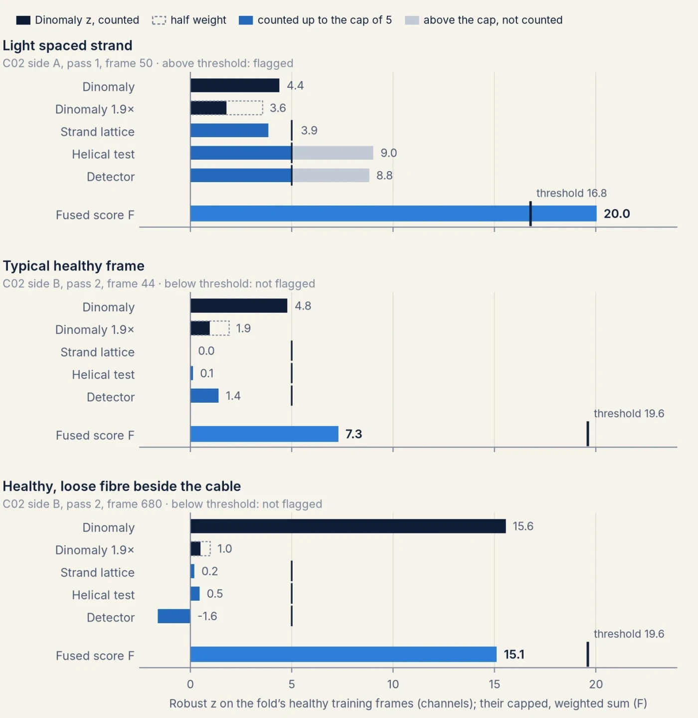
Cost
Every component was timed on the same machine, one NVIDIA H100 (80 GB) with 8 physical CPU cores, on one fold (cable 2, fold 0: 100 training and 1,199 test frames), one component at a time.
| Per fold | Hardware | Train | Score test frames |
|---|---|---|---|
| Dinomaly | H100 | 96 s | 20 s |
| Dinomaly at 1.9× | H100 | 92 s | 35 s |
| DINOv3 detector | H100 | 377 s | 91–120 s |
| Strand lattice | 1 CPU core | 72 s (normal model and scoring) | |
| Helical test | 1 CPU core | 102 s (normal model and scoring) | |
| Fusion and threshold | 1 CPU core | about 1 s | |
| Per frame, once, shared by all folds | Hardware | Time |
|---|---|---|
| Aligned view | 1 CPU core | 0.13 s |
| Tiles at 1.9× | 1 CPU core | 0.06 s |
| Detector strip | 1 CPU core | 0.28 s |
| Lattice geometry | 1 CPU core | 1.04 s |
| Helix fit and groove measurements | 1 CPU core | 3.94 s |
A fold therefore costs about 12 minutes of H100 time, two thirds of it the DINOv3 detector, plus about 3 CPU-core minutes; the geometric channels are single-threaded per fold, so folds run side by side. The per-frame preprocessing totals about 5.5 CPU-core seconds per frame, most of it the helix fit. Dinomaly is scored in fp32 and trained in bf16; the detector scores frame by frame. For reference, one Dinomaly fold takes about 8 minutes on an NVIDIA A10G.
4Evaluation protocol
The benchmark is a k-fold, few-shot protocol. There are 116 folds, 40, 46 and 30 for the three cables. Each fold gives 100 healthy frames to train on, and its test set is the healthy and damaged frames from the rest of that cable. No defect labels are allowed at training time. Metrics are image-level: AUROC, the probability that a damaged frame scores above a healthy one; AUPR; and F1 and false-positive rate at a threshold chosen without test data. Each cable’s folds are averaged first, and results are reported as mean ± standard deviation across the three cables.
We kept all of its rules and added our own, fixed before any run:
- Per fold, only that fold’s data. Its 100 healthy frames, synthetic data made from them, and external non-CableInspect data such as pretrained weights. Never real defect pixels, other folds’ frames, or neighbouring frames or passes at test time.
- Choices on development folds. Four folds per cable for every tuning decision; the benchmark’s fold files are used unchanged.
- A sealed cable. The final method was developed by AI coding agents working in sandboxes that held only cables 1 and 2: no image, label or fold file of cable 3, and no result on it. Their full command logs, and the machines they used, were audited for any contact with cable 3 before it was run. The remaining folds of cables 1 and 2 served as an internal check, looked at once per frozen version. Each frozen version was then run once on cable 3 by a separate evaluation agent that computed no metric; which version to evaluate was decided on cable 1 and 2 evidence only and logged first.
- Every score kept. Per-image scores of every fold of every method are saved, so any metric can be recomputed.
The 116-fold numbers therefore include two cables the method was developed on; on those cables, its holdout folds were looked at once per version. To test cables 1 and 2 cleanly as well, the sealed setup of rule 3 was repeated for each of them. Two further teams of agents each worked in a sandbox without one cable, starting from the method’s code with every mention of that cable removed and no result on it. Each re-made the method’s data-dependent choices on its two visible cables and froze a recipe. Their command logs were audited as in rule 3. An evaluation agent checked the frozen code on the scoring machines and reproduced every channel and the fusion byte for byte on a fold of a visible cable. It then ran the recipe once on all folds of the hidden cable. Cable 3 keeps its result from rule 3. As in the protocol, each cable’s folds are averaged, then the three cables count equally.
5Results
Every cable held out
The cleanest test of a method is a cable its developers never saw. Cable 3 was held out from the start (below). Cables 1 and 2 were each held out from a new team, which re-made the method’s choices on the other two cables (section 4).
Each held-out cable was run once with a recipe frozen without it. “As dev cable” is the method of section 3 on the same cable in the 116-fold table, where cables 1 and 2 were development cables. The matched Dinomaly was tuned and frozen without the held-out cable: by the same team for cables 1 and 2, and by the earlier sealed agent of Figure 12 for cable 3. F1 and FPR are at the recipe’s own frozen threshold. Intervals resample the cable’s folds, which share most of their test frames, so they describe stability on that cable. They are not replicates over cables.
On cables 1 and 2 the held-out recipes score 0.979 and 0.950. The method of section 3 scored 0.979 and 0.952 on them when they were its development cables, so developing on these cables raised their scores very little. Over the three held-out cables the mean is 0.951 ± 0.027, with AUPR 0.966. The fusion beats the matched Dinomaly on every fold of cables 1 and 2 and on 27 of 30 of cable 3, by 0.019 on average. Light spaced strands rise from 0.751 to 0.895.
The two new teams kept the five channels and the form of the fusion, and re-made their settings. The team without cable 1 uses a ViT-L Dinomaly trained for 500 steps. It weights the two geometric channels 0.75 and Dinomaly at 1.9× 1, and places half of its drawn scratches and speckled deposits on the cable’s outline. The team without cable 2 weights every channel 1. Both cap the specialist channels at 8 instead of 5 and score the detector with five cross-fitted heads. Both also use more helical features than section 3, and fitted their own margins (2.35 and 2.41; 2.64 and 2.69). The result therefore tests whether the way the method is developed carries over to a cable its developers never saw. It is not a test of one fixed recipe. The method family itself, including the aligned view and the first defect generators, was shaped earlier with all three cables in view (Appendix D). Per-channel and per-kind results of the held-out recipes are in Appendix C.
Ranking aside, an inspector needs an operating point. Fixing the share of defect frames to find, per fold from the test labels (a diagnostic, not a usable rule), shows what the ranking allows. To find 80% of defect frames, the held-out recipes flag 4.2% of healthy frames, against 7.5% for the matched Dinomaly. At 90% recall they flag 16.6% against 24.6%. At 95% both flag a third or more: the last defect frames, short gaps at the frame edge and faint marks, are hard for every method.
The frozen threshold misses its target on every held-out cable. It is set to flag 5% of healthy frames, and flags 8.9%, 8.8% and 12.2% of them on cables 1, 2 and 3. Both new teams had found the same problem on held-out folds of their visible cables before freezing (7.6% and 9 to 10%).
Healthy test frames flagged at each recipe’s frozen threshold, averaged over folds, split by whether the frame’s side and pass occur among the fold’s 100 training frames; “of n” is the mean number of such frames per fold. Some folds have no healthy test frames outside their training sides and passes: 4 of 46 on cable 2 and 5 of 30 on cable 3. Computed after the fact from the saved scores; no setting was changed.
The misses are not only on new camera passes. On cables 1 and 2, healthy frames from a side and pass absent from the training frames are flagged more often (10.8% and 9.5%, against 5.6% and 6.9%), so the larger margin for those frames does not fully cover them. On cable 3 the pattern reverses: frames from a side and pass the training frames include are flagged most (15.1%, against 9.1%). The misses are also uneven between folds: 14 of 40, 14 of 46 and 16 of 30 folds flag over 10%, and single folds reach 43%. This fits the explanation in the threshold section: healthy stretches of cable that look unlike the fold’s training stretch score high, whether or not the pass is new.
All 116 folds
Our method scores 0.979, 0.952 and 0.924 on the three cables, 0.952 ± 0.028 overall, with AUPR 0.967, against 0.931 for tuned Dinomaly on the same view and 0.86 for the best published method.
Cable 3 in detail
On cable 3 our method scores 0.924, +0.015 over the same-conditions Dinomaly on 27 of 30 folds. Adding the learned detector gains +0.004 on cable 3, at least as much as on the held-out folds of the development cables (+0.0022 and +0.0026). Light spaced strands rise from 0.687 to 0.914; light scratches, partial broken strands and light crushing remain below Dinomaly alone (section 6).
The 95% intervals in Figure 12 resample the 30 folds of cable 3, and those folds share most of their test frames and the same cable. They therefore say how stable the comparison is on this cable, not how well it would carry over to a new one. The held-out recipes above extend the test to the other two cables.
Each method’s F1 and false-positive rate in Figure 12 come from its own threshold rule, so they compare rules as much as models. A rule-free comparison is the share of healthy frames a method must flag to find a given share of defect frames, set per fold from the test labels and averaged over the 30 folds (diagnostic only):
| Cable 3, healthy frames flagged at a fixed defect recall | 80% recall | 90% recall | 95% recall |
|---|---|---|---|
| Ours | 7.4% | 31.1% | 52.8% |
| Ours without the DINOv3 detector | 7.4% | 34.0% | 55.5% |
| Strand lattice + Dinomaly | 8.9% | 36.3% | 55.7% |
| Dinomaly | 14.3% | 38.4% | 53.9% |
At 80% recall our method flags half as many healthy frames as Dinomaly. At 95% the methods are level: the last few defect frames, mostly short gaps at the frame edge and faint surface marks (section 6), are as hard for every method.
What each channel contributes
Computed after the fact from the saved per-frame z-scores of the frozen method, by removing one term of the fused score and keeping the others’ weights; nothing was re-tuned, and no choice was made from this table.
The two geometric channels together are worth +0.010 over all folds, more on the development cables than on cable 3. Removing Dinomaly costs most on cable 3, 0.020. The DINOv3 detector adds +0.003 overall. The strand lattice is the exception: without it, cable 3 would score 0.927 instead of 0.924, so it helps on the development cables and slightly lowers the score on the unseen one.
The aligned view, for every method
Part of the gain could come from more pixels on the cable. A resolution ablation with PatchCore separates the two effects: doubling the resolution or tiling is worth about +0.015, whereas aligning the cable at the same resolution per tile is worth about +0.06.
The threshold
AUROC does not depend on the threshold. Every method here sets its threshold from the fold’s healthy training frames, so one fixed rule gives different false-alarm and miss rates from fold to fold.
Ours · threshold: margin rule fitted on dev folds · mean of cables 10% flagged, 17% missed
Dinomaly at the paper’s rule flags 12% of healthy frames but misses 40% of defect frames. Without its learned detector, our method’s margin rule flags 6.3%, 6.0% and 5.7% of healthy frames on the three cables, the unseen cable included, and misses 19%. With the detector it misses fewer (17%) but flags more, 9% on the development cables and 12% on cable 3: the margins fitted on the development folds do not fully carry over once the detector is added. Scoring all 100 training frames out of sample, with five cross-fitted detector heads, did not lower it, so the cause is not the size of the detector’s healthy reference but that healthy frames from other stretches and passes do not look like a fold’s training stretch. The held-out recipes, with margins fitted by their own teams, miss in the same way (8.9% to 12.2%, above). The rule has no formal guarantee; it has only been checked on these folds.
Reproducing the published baseline
The paper’s Enhanced-PatchCore row is AUROC 0.78. Our first reproduction came out higher, at 0.825, and the difference was a single line of preprocessing: the bilinear resize without anti-aliasing. Doing the same reproduces the published row.
We cannot explain why the published spread across cables (0.05) is so much larger than ours (0.006).
6Remaining errors
Light damage
Every severe grade scores 0.98 to 1.00; the errors are in light damage. On cable 3 alone, the clean test, the pattern is the same and sharper:
Cable 3, 30 folds, run once. Healthy frames against frames showing only that kind and grade. Dinomaly is the same-conditions Dinomaly of Figure 12; “without detector” is our method without its DINOv3 channel. Kinds with fewer than 6 frames per fold (the welded grades) are left out.
Light spaced strands rise from 0.687 for Dinomaly to 0.914, important spaced strands from 0.898 to 0.975 and extracted strands from 0.943 to 0.960. Faint surface damage goes the other way: light scratches 0.828 against 0.874, partial broken strands 0.773 against 0.835, light crushing 0.894 against 0.906 and light deposits 0.814 against 0.820. The geometric channels lift some healthy frames above these faint marks; the DINOv3 detector wins part of it back (light scratches 0.810 without it, 0.828 with it). Light spaced strands improve on every held-out cable (section 5): 0.924, 0.846 and 0.914 on cables 1, 2 and 3, against 0.834, 0.731 and 0.687 for the matched Dinomaly. Cable 2 remains the hardest.
Where the missed defects and false alarms are
To see what limits the ranking, we charged each misordered (defect, healthy) frame pair half to each frame, on the held-out folds of the development cables for an earlier fusion with the same geometric channels.
- Missed defects are mostly short spaced strands at the frame edge. Light spaced strands carry about half of the defect side of the loss (54% on cable 1, 46% on cable 2), in boxes 150 to 450 px wide on a 1,920 px frame, and about 56% of that comes from gaps that touch the left or right edge of the frame. Below about 300 px of visible gap, further changes to the helical channel did not help: healthy cable shows openings of the same shape, and a whitened matched filter added nothing. The neighbouring frames that show the rest of the gap are off limits under the protocol.
- False alarms are healthy frames with scuffs or loose fibres. The worst tenth of healthy frames per fold carries about half of the healthy side. They come in runs of consecutive frames along scuffed but healthy stretches (one pass of cable 1 alone carries 38%), and on cable 2 several are loose fibres lying on the background next to the cable.
Tried and dropped
On the development folds, these did not improve the fusion: physically rendered defects (a classifier still tells them from real ones at 0.98), pixel-level appearance models, a likelihood ratio learned from simulated gaps, learned fusion weights, a deposit generator modelled on a review of missed deposits, and five cross-fitted detector heads in place of one (which rank about the same).
7Discussion and conclusion
With every cable held out from its developers our method scores 0.951 AUROC, and 0.952 over all 116 folds of the published protocol, against 0.86 for the best published result and 0.931 for the best of thirteen recent methods we re-ran under identical conditions. Three contributions produce that, and they are not equally established.
- The aligned view is the largest and most general gain. Rotating, scaling and normalising the cable from each frame alone raises Dinomaly from 0.891 to 0.931 and ten of twelve detectors by 0.022 to 0.062, across method families. It costs about 0.13 s per frame on one CPU core and needs no labels.
- Corrections to the evaluation. A one-line resize difference explains the published PatchCore row; thresholds fitted on a trained model’s own training frames are biased low; anomalib 2.7 steps three methods’ learning-rate schedules once per epoch; and split-conformal thresholds fail here because a fold’s healthy frames are one stretch of cable. These hold independently of our method.
- The fusion adds 0.021 over tuned Dinomaly over all folds and 0.019 over the matched Dinomaly on the three held-out cables, with strand geometry for the spaced strands that reconstruction misses and a detector trained against hard healthy examples. A frozen backbone larger than ViT-L did not help, and a fine-tuned one added nothing.
The held-out score, 0.951 ± 0.027, is within 0.002 of the method’s scores on the cables it was developed on. Developing on cables 1 and 2 therefore did not noticeably inflate the 116-fold result. Two limits remain. First, each held-out cable had its own frozen recipe: the way the method is developed carries over, which is not the same as one recipe carrying over. Second, the method family, including the aligned view and the first defect generators, was designed earlier with all three cables in view. The intervals resample folds of one cable, which share frames, so they are not replicates over cables. With three cables there is little to say about a fourth.
The threshold is the open problem. Set to flag 5% of healthy frames, it flagged 8.9%, 8.8% and 12.2% on the held-out cables, and up to 43% on single folds. The ranking would allow better: at 80% defect recall the held-out recipes flag 4.2% of healthy frames. The misses come from healthy stretches unlike the fold’s training stretch, on new camera passes and familiar ones alike. A fold’s 100 healthy frames come from one stretch of cable, and a threshold fitted only on them does not say how healthy frames elsewhere will score.
The hand-built parts of the method should be read in the light of the bitter lesson:8 methods that encode knowledge of a domain tend to be overtaken by general methods that learn it from more data and compute. The strand-geometry channels, the defect generators and the constants of Appendix D are such knowledge, and the lattice channel’s cost on the unseen cable is the kind of failure to expect from them. They pay here because the benchmark is small: a fold gives 100 healthy frames of one stretch of cable, no defect labels, and only three cables exist. Our own results point the same way. A larger frozen backbone did not help and fine-tuning one learned the drawn defects instead of real damage, which is what too little data looks like rather than too little capacity. With more cables, more healthy footage or labelled defects, we would expect a general learned detector to generalise better than these channels and to make most of them unnecessary; the benchmark does not provide that data.
One further limitation is faint surface damage. Light deposits score below Dinomaly alone on all three held-out cables (0.936, 0.950 and 0.814 against 0.948, 0.961 and 0.820). Light scratches and partial breaks are behind clearly only on cable 3: on held-out cables 1 and 2 the fusion is level on scratches and ahead on partial breaks.
Appendix
A · Earlier versions and the first sealed tests
Before the final method we built a synthetic-defect detector on frozen DINOv2 ViT-S tokens of the aligned view (v2), trained on defects drawn in code and fused with tuned Dinomaly (0.939 over 116 folds, best when it was frozen). Its later configurations were shaped by looking at test errors and are listed but not counted. To test it on an unseen cable, three AI coding agents each rebuilt it in a sandbox holding only two cables and froze it before a single run on the third. Each beat its own Dinomaly on the unseen cable by +0.003 to +0.009, less than on its development folds (+0.010 to +0.017). A fourth agent without cable 3 took a different route, the strand lattice now used as a channel, and reached the same 0.916 on cable 3.
F1 and FPR at each agent’s own frozen threshold rule. The mean row averages the three cables, one agent each.
B · Three implementation details in the re-run baselines
- A learning-rate schedule stepped once per epoch. anomalib 2.7 returns the schedulers of Dinomaly, INP-Former and EfficientAD without
"interval": "step", so Lightning steps them once per epoch. With 100 training frames an epoch is only 6 steps, so Dinomaly’s learning rate is zero for the first 6 steps and never rises above half its base value. Our tuned runs step per batch, as the official code does. - Half-precision scores tie. The bf16 Dinomaly scores took about 400 distinct values over 65,695 frames, and the fp16 SuperSimpleNet scores saturated near 1.0 for 28 to 36% of defect frames. Every number on this page is scored at full precision.
- Trained models score their own training frames too low. We hold out 20 of the 100 frames for every trained model to fit its threshold on.
C · All numbers
Image-level metrics over all 116 folds unless stated; mean ± std across cables after averaging each cable’s folds. Run names refer to the wandb project. The held-out results were scored and analysed from saved per-frame scores and are not logged to wandb; their score files, frozen recipe archives and checksums are kept with the analysis.
Thirteen methods, both inputs
F1 and FPR at the beta-prime threshold. Trained models fit it on 20 training frames held out of training; training-free anomalib models score each training frame with a model built from the other four fifths; memory banks hide a frame’s own patches.
Per kind of defect, all 116 folds
Paired differences over folds
Difference = mean over cables of each cable’s mean per-fold AUROC difference; 95% interval from 10,000 resamples of folds within each cable.
Per physical defect, earlier fusion
Mean over each cable’s folds, then over cables; about 125 visits and 50 physical defects per fold. The 5% points are set on each fold’s healthy test frames, so they are diagnostic only.
Held-out recipes, each channel alone
Image AUROC of each channel’s own score on its held-out cable, mean over the cable’s folds. Cables 1 and 2 are the recipes of the teams without them; cable 3 is the method of section 3. The detector channel of the two new recipes uses five cross-fitted heads.
Held-out recipes, per kind of defect
Healthy frames against frames showing only that kind and grade, on each held-out cable, ours against the matched Dinomaly. A cable is left out for a kind with fewer than 6 such frames per fold.
D · Settings and where they were chosen
Every setting of the method, grouped, with the data it was chosen on. “Dev folds” means the four development folds of cables 1 and 2; nothing below was chosen on cable 3.
| Component | Settings | Chosen on |
|---|---|---|
| Aligned view | green-screen test (1.12, 20), cable thickness 224 px, exposure target 160 with gain in [0.6, 1.6], 40 px loose-piece size, four tiles | Designed before the sealed rounds, with all three cables in view; unchanged since |
| Dinomaly 1× | ViT-B/14, 448 px tiles, 1,000 steps, batch 16; anomalib defaults otherwise | Dev folds, by an earlier agent without cable 3 |
| Dinomaly 1.9× | crop of rows 106–342, 7 tiles; same Dinomaly settings | Dev folds |
| Strand lattice | unwrap range, blur scales, groove tracking, ribbon size, ±4 periods, cell size, 12 features, clip limits | Dev folds, by an earlier agent without cable 3 |
| Helical test | camera-distance set, lattice search range, sampling step and averaging, five features and three sums, AR order, angle bins, CUSUM steps | Dev folds |
| DINOv3 detector | backbone and blocks, head, crop size, steps, loss weight and k, frame aggregation, end-crop share, negative marks | Dev folds |
| Drawn defects | the 2D defect and wear generators reused by the detector | Designed in an earlier round with all three cables in view, each from one real example per kind; the warp-based strand and speckle families are new and chosen on dev folds |
| Fusion | weights (1, 0.5, 1, 1, 1), caps at 5 | Dev folds |
| Threshold | α = 0.05, margins 2.31 and 3.13 | Dev folds |
The two rows designed with all cables in view remain test-informed. The held-out recipes of section 5 re-made every setting below except those two rows, on the two cables each team could see. Their choices differ from this table where stated there.
References
- Arodi, Luck, Bedwani, Zaimi, Li, Pouliot, Beaudry and Marceau Caron. CableInspect-AD: An Expert-Annotated Anomaly Detection Dataset. NeurIPS 2024 Datasets and Benchmarks Track. arXiv:2409.20353. Project: mila-iqia.github.io/cableinspect-ad. Data: Hydro-Québec open data; the licence file in the release is CC BY-NC-SA 4.0.
- Roth et al. Towards Total Recall in Industrial Anomaly Detection (PatchCore). CVPR, 2022.
- Oquab et al. DINOv2: Learning Robust Visual Features without Supervision. TMLR, 2024.
- Akcay et al. Anomalib: A Deep Learning Library for Anomaly Detection. ICIP, 2022. Version 2.7.0 provides SuperADD, RAD, Dinomaly, INP-Former, GLASS, EfficientAD, FoundAD, SuperSimpleNet, AnomalyVFM and MH-PatchCore as used here.
- Lu and Shao. A framework for unsupervised anomaly detection in real-world cable inspection. Signal, Image and Video Processing 20:33, 2026. doi:10.1007/s11760-025-05087-3. Cited, not run: its abstract gives no absolute numbers.
- Siméoni et al. DINOv3. arXiv, 2025.
- Vovk, Gammerman and Shafer. Algorithmic Learning in a Random World. Springer, 2005.
- Sutton. The Bitter Lesson. 2019. incompleteideas.net.
Cite this
@misc{headroomgrid2026cableinspect,
  title  = {Finding damaged strands on power cables},
  author = {{Headroom Grid}},
  year   = {2026},
  month  = oct,
  note   = {CableInspect-AD: strand geometry and a frozen foundation model, fused; each cable held out from its developers},
  url    = {https://headroomgrid.eu/research/cableinspect-ad/}
}
Images and labels: CableInspect-AD, Arodi et al. 2024, by Hydro-Québec and Mila, licensed CC BY-NC-SA 4.0 (the Hydro-Québec download page names CC BY-NC 4.0). The frames and tiles on this page are resized and cropped from that release and shared under the same licence, non-commercially, with maps of our models.