Reading open trenches in 3D: A pretrained encoder for underground utility mapping
Pipes and cables underground can only be seen when the trench is open. Recording them keeps underground utility registers accurate. OpenTrench3D, 310 smartphone scans of open trenches in Denmark, is a public dataset that benchmarks how to do this accurately.
The best published method scores 84.8 out of 100 on the benchmark’s accuracy measure (mIoU). We fine-tuned an open-source model, Utonia, on OpenTrench3D to reach a new published state of the art on this benchmark of 88.0 mIoU. Our ablation shows Utonia's pretraining data is a major source of the improvement. Furthermore, we show that current methods do not use the same evaluation protocol, and this difference explains part of the progress reported so far. We report our results on both evaluation protocols.
The results of this work can improve localisation and registration of underground utilities. Additional retraining will likely be required in environments outside the current training distribution.
Loading scan…
1The dataset
OpenTrench3D is a dataset of 310 scans of open trenches in Denmark, totalling 528 million points.1 The scans were registered with a smartphone, and then transformed into point clouds, accurate to roughly ±5cm. Each point has one of five labels: main utility, other utility, inactive utility, trench (soil, walls, surroundings) and misc (ignored by every benchmark). Scans form two groups:
- Water Areas: 260 trenches are water pipes (filmed across five different areas) with 35 to 68 scans each.
- District Heating: 50 trenches for district heating.
2Prior work
Methods evaluated on OpenTrench3D
The baselines of the dataset paper use models derived from PointNet++.11 These networks assign class scores to every point with an encoder-decoder architecture. In PointNet++, at the first encoder stage, each neighbour point of a sampled centre is represented by its three coordinate offsets from that centre and three RGB colour values. A shared MLP transforms each vector into a learned feature vector. Component-wise max pooling is then applied to the set of feature vectors in the neighbourhood to produce one vector per neighbourhood. By repeating this procedure, where sampled centres become the input points for the next encoder stage and learned feature vectors replace RGB values, each group covers a larger region as the neighbourhood radius increases.
The decoder then reverses this by interpolating feature vectors from the sampled centres back to the points present before each sampling step. Each point receives a weighted average of the vectors at its three nearest centres, with weights proportional to inverse squared distance. This vector is then concatenated with the encoder vector retained for that point via skip connections, and passed through a shared MLP. The process repeats until every original point has a feature vector. A final shared classification MLP then predicts class scores for each point; the network is trained using cross-entropy loss.
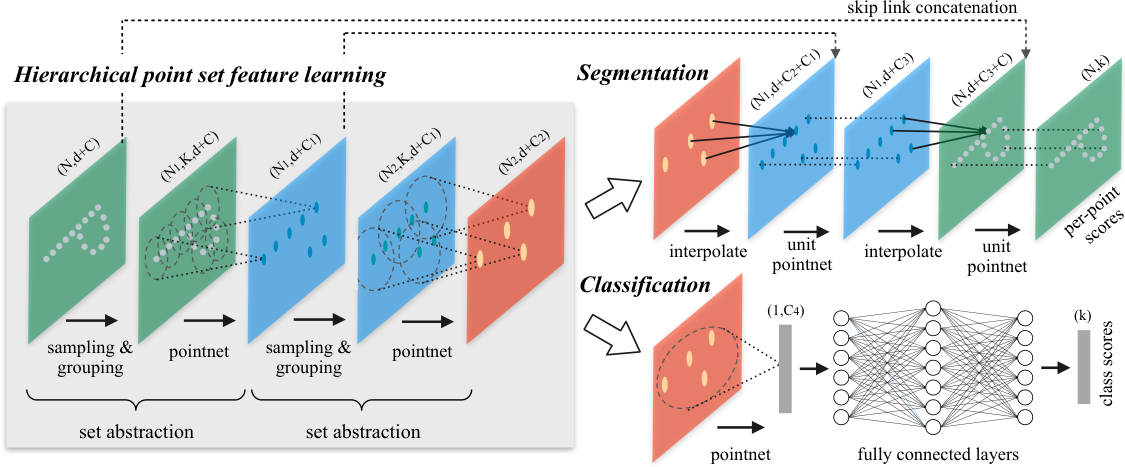
Hansen et al. introduce the OpenTrench3D dataset and train three PointNet-like models on it.1
Liu et al. use a transformer-based point architecture that combines neighbouring points' feature vectors with attention weights. In addition, they group feature channels so multiple channels share attention weights and can exchange information between groups through their Group-aware Channel Interaction Module (GCIM). They make attention depend on position by adding a term that combines the two points’ feature vectors with their coordinates and the difference between their indices in the spatially ordered point sequence. They train the network on Water Areas 1–4 and test it on Water Area 5, reporting 84.8 mIoU, the best published result on that split.2 Unlike Hansen et al., they do not use five-fold cross-validation, making it harder to compare the two methods directly. Both methods report single-run numbers and use networks trained with randomly initialised weights.
Approaches to point-cloud segmentation
Semantic segmentation of point clouds has developed along three architectural lines. Point-based networks, described above, work on the raw points and summarise neighbourhoods at several scales. Sparse convolutional networks voxelise the cloud and apply convolutions only at occupied voxels, which keeps the computation proportional to the surface rather than the volume, in U-Net encoder–decoders.12,13 Point transformers replace convolution by attention: Point Transformer attends over the k nearest neighbours of each point;14 Point Transformer V3 orders the points along space-filling curves (Z-order and Hilbert) and attends within patches of consecutive points, which widens the receptive field at lower cost and lets the model scale.3
Labelled 3D data is scarce, because every point has to be annotated, and high-capacity models such as point transformers need more of it than a single benchmark provides. The best results on indoor benchmarks such as ScanNet and S3DIS18,19 now come from self-supervised pretraining: the encoder is first trained on many unlabelled scans, then fine-tuned on the target task with the labels available. Three successive models from the Pointcept group5 follow this route, all with a Point Transformer V3 encoder.
Sonata learns by self-distillation. A student encoder sees local crops and masked versions of a scene, and a teacher, whose weights are an exponential moving average of the student’s, sees the full scene. The student is trained to assign each point to the same learned prototypes as the teacher. The encoder is pretrained without a decoder, which the authors found keeps its features from collapsing onto point positions.4
Concerto keeps this objective and adds a cross-modal one. Its scenes come with posed images, each encoded by a frozen DINOv217. The 3D features of the points that project into an image patch are averaged and trained to predict that patch’s DINOv2 feature under a cosine loss. Concerto is pretrained on about 40,000 indoor point clouds with 300,000 images and fine-tunes to 80.7 mIoU on ScanNet.16
Utonia trains one encoder with both objectives across five domains at once: indoor RGB-D scans, outdoor LiDAR, remote sensing, point clouds lifted from video, and single objects, about 250,000 scans and a million objects in all. Two changes make the domains compatible. First, every cloud is rescaled to a shared granularity before the voxel grid and the 3D rotary position encoding are applied, so a room, a street and an object reach the attention layers at comparable scales. Second, colour and normals are dropped at random during training, so the encoder still works where a domain lacks them. The released encoder is a Point Transformer V3 of 137 million parameters, with five stages of 54, 108, 216, 432 and 576 channels and 3, 3, 3, 12 and 3 blocks, attending within patches of 1,024 consecutive points along the space-filling curves. It fine-tunes to 81.1 mIoU on ScanNet and 78.1 on S3DIS.5,15
4Evaluation protocol
The literature reports two different evaluation protocols. In the first setting, we use a five-fold cross-validation over the water areas, leaving out one area for evaluation and training on the remaining sections. This is the protocol that is used by the original dataset authors. The second protocol simply trains on Water Areas 1-4 and evaluates on Area 5. We report our results in both settings.
Since 92.6% of the points in Water Area 5 are trenches, a model that classifies each point as trench is 92.6% accurate. The evaluation is therefore the mean intersection-over-union (mIoU) over the four classes (main/other/abandoned pipes, trench), weighing each class equally irrespective of the number of points. In practice, we expect utility operators to care mostly about the pipes found. Hence, we simply report pipe count as well, where we define a pipe as found when half of its ground truth points are classified as such by the model.
Current evaluation protocols do not provide results for heating-area scans. We report the defined metrics on these areas separately to maximise insights from the available data.
3Approach
Our main contribution is simple: general pre-trained point cloud networks outcompete models only trained on OpenTrench3D. This is not surprising given that large-scale pre-training has been a proven recipe for many years. We evaluate the three pre-trained models mentioned above: Utonia, Sonata and Concerto.
Utonia pre-training data contains indoor object datasets, driving LiDAR, areal scans and house tours, but no trench data.
Model
We use Utonia’s released encoder unchanged. Our decoder has four stages with two blocks each, from 432 down to 54 channels, connected to the encoder by skip connections. Finally, we add a linear head that maps each point’s 54-channel feature to the four classes. Decoder and head are initialised from scratch; stochastic depth is 0.3.
Data and input
Each point enters with its coordinates, its colour and a surface normal estimated from its neighbours within 3 cm (at most 30). For the Water Area 5 benchmark the model trains on the 210 scans of Water Areas 1–4; for each cross-validation fold, on the four other water areas. Training reads a 1 cm copy of the release; coordinates are halved, Utonia’s convention for indoor scenes, and voxelised so that one point is kept per 2 cm voxel, and a random crop keeps at most 102,400 points, which covers most scans whole. Misc points are excluded from the loss. Each training sample is augmented: 20% of its points are dropped at random, it is rotated about the vertical axis by a random angle and tilted by up to 2.8° about each horizontal axis (each with probability 0.5), scaled by a factor between 0.9 and 1.1, mirrored with probability 0.5, and every point is moved by up to 5 mm. Colours are perturbed by an occasional auto-contrast, a global shift of up to 5% and per-point noise. With probability 0.8, two training scans are merged into one sample.
Training
As in Utonia’s published fine-tuning recipe, the loss is cross-entropy plus the Lovász-softmax loss, a differentiable surrogate of IoU, with equal weights.10 We optimise with AdamW (weight decay 0.01) at a peak learning rate of 0.001 for the new decoder and head and 0.0001 for the pretrained encoder blocks, on a one-cycle schedule: linear warm-up over the first 5% of steps from a tenth of the peak, then cosine decay. Training runs for 300 passes over the training scans at batch size 4, in mixed precision with gradients clipped at norm 3. Every setting is trained with three seeds and reported as their mean ± standard deviation. A run saves the model after each of its ten training cycles, and we always test the model from the end of training. Picking whichever saved model scores best on the test area would use the test data to make a choice, and would inflate the result. Averaging the last three saved models was no better on the development split, at 79.3 against 79.6 (both tested at full resolution on Water Area 4).
Inference
A test scan is processed whole, without cropping. It is read at the full 4 mm resolution and voxelised to 1 cm. Several 2 cm voxelisations then cover it, so that every 1 cm point is predicted once. Each prediction is copied to all original points in its voxel, so the metrics count every point of the release. Test-time augmentation (13 views: rotations about the vertical axis, rescalings and a flip) adds 1.4 to 1.6 points. It is reported separately, and the headline numbers are without it. On one NVIDIA L40S GPU, labelling a scan of about 1.6 million points takes about one second in a single pass, and training one model takes about four and a half hours. The network has 158 million parameters, against 24 million for PointVector-XL8.9
5Results
Development split: choosing the backbone
We compared three self-supervised Point Transformer V3 backbones from the Pointcept group: Sonata, Concerto and Utonia.3,4,5,15,16 Each ran with its own published fine-tuning settings, and we chose the one with the highest mean validation mIoU over the last three of ten training cycles, since a single cycle can swing by up to 6 points. Had the scores fallen within 0.5 points of each other, we would have kept Sonata as the simplest.
Utonia led from the second cycle onwards and scored 78.16, against 69.98 for Sonata and 69.53 for Concerto. These are the training code’s own validation scores, computed on a 1 cm copy of Water Area 4; testing the final checkpoint at full resolution with our evaluator gives 79.6, the figure compared with weight averaging in section 3. The rise over the last cycles comes from the learning-rate decay at the end of the schedule, not from training too short: doubling the schedule to 600 passes scored 80.9 against 81.2 mIoU over the four folds (Appendix B).
Water Area 5
We trained three seeds on Water Areas 1–4 and tested each once on Water Area 5. All three beat the previous best, the lowest scoring 87.5, and with test-time augmentation the mean rises to 89.6 ± 0.5. Averaging the three seeds’ augmented predictions, an ensemble reported separately, gives 90.0 and finds 266 of the 275 pipes, against 265–267 for the single seeds.
Water Area 5 split train Water 1–4, test Water 5
Five-fold cross-validation mean over the five water areas
Pretraining versus training from scratch
To separate pretraining from architecture and size, we trained the same network from random initialisation: Utonia’s architecture and parameter count, its published recipe and the same 300 passes on Water Areas 1–4, with one learning rate of 0.001 for all parameters, since the lower rate for encoder blocks only exists to protect pretrained weights. Two seeds score 79.4 and 81.2 on Water Area 5; a third diverged during training (53.7, after repeated numerical overflow) and is reported but not averaged. With pretraining the same network scores 88.0 ± 0.7. Without it, it falls below PointVector-XL8, which averages 85.0 on the same split with 24 million parameters against 158 million for our network. Model size alone therefore does not explain the gain; most of it comes from the pretrained weights. The initial from-scratch runs reused the fine-tuning recipe without tuning it for random initialisation. We then compared four learning-rate and schedule settings on Water Area 4, without using Water Area 5, and selected 600 passes with a peak learning rate of 0.0005 for all parameters. On Water Area 5, that setting scores 82.9, 81.9 and 84.0 across three seeds (82.9 ± 1.1). This is 5.1 points below the pretrained mean of 88.0 and 2.1 below PointVector-XL’s 85.0. The scratch result makes the size comparison more informative: the same 158-million-parameter architecture, after modest recipe tuning, still scores below both pretrained models.
Effect of the test area
Liu et al. compared their Water Area 5 result with the dataset paper’s five-fold numbers. To see what the split alone does, we retrained two of the paper’s baselines on Water Area 5 with the paper’s settings. PointNeXt-XL rises from 70.6 to 81.5, and PointVector-XL from 76.5 to 84.1 with one seed; over three seeds PointVector-XL averages 85.0, above the 84.8 of the previous best.7,8
Tested on Water Area 5 rather than averaged over five areas, the same networks with the same settings score 10.9 and 7.6 points higher. Water Area 5 is easier than the average: in our own five-fold run it scores 88.0, against 76.6 on the hardest area. The 8.3-point gain that Liu et al. report over PointVector-XL (84.8 against 76.5) comes from the choice of test area: on the same split, PointVector-XL averages 85.0 over three seeds. Our own margin over it on that split, three seeds each, is 3.0 points.
We also compared the two scan by scan, with three retrained PointVector-XL seeds (84.1, 85.5, 85.2; 85.0 ± 0.7). On the 50 Water Area 5 scans our seed mean scores higher on 40 and lower on 10; resampling the scans 10,000 times gives +3.0 mIoU with a 95% interval of −0.0 to 6.6, and +10.3 (0.1 to 22.2) on abandoned pipes. Fifty scans are too few to settle a gap of this size. We therefore trained PointVector-XL with the same settings on the other four folds as well and repeated the comparison over all 260 water scans, each tested by a model that never saw its area. There the mIoU pooled over all 260 scans is 81.7 for our model and 76.3 for PointVector-XL, a difference of +5.4 (95% interval 3.7 to 7.1); scored scan by scan, our model is higher on 184 of the 260; per class, main +3.6 (2.0 to 5.4), other +1.3 (−0.6 to 3.2) and abandoned +16.4 (11.8 to 21.3). PointVector-XL has one seed on Water Areas 1–4, so these intervals cover variation between scans but not between its seeds. Liu et al. have not released code, so their numbers cannot be checked, and we report them as published.
Per-class results
Our model scores higher than every published method on all four classes, although trench is close to its ceiling for every method. The gain is largest on abandoned pipes, at 71.3 against 65.6 (76.0 with TTA), and this class also accounts for most of the spread between seeds, which score 75.6, 68.9 and 69.5 on it.
Five-fold cross-validation
Each water area serves once as the test area, with training on the other four and three seeds per fold. The mean is 81.6 ± 0.7 over seeds (83.0 ± 0.3 with TTA), against 76.5 for the best published result, PointVector-XL. Retrained by us on the same folds, PointVector-XL averages 76.6 (one seed per fold on Water Areas 1–4, three on Water Area 5), which matches the published number. Water Area 4 was our validation area during development, so its fold may flatter the model; without it the mean is 82.8.
Fold means range from 76.6 to 88.0, while the seeds within a fold stay within 2.4 points of each other. The two lowest folds are also the lowest on abandoned pipes: 51.3 IoU on Water 1 and 42.1 on Water 4.
Transfer to district heating
The third benchmark tests how well a model transfers from water trenches to district-heating trenches when only a few labelled scans are available. As in the dataset paper, whose baselines were also trained on the water areas first, we start from our Water 1–4 model, fine-tune it on 1 to 29 scans of Heating Area 1 and test on Heating Area 2 with three classes (abandoned pipes are not scored). The from-scratch square in the figure is the paper’s baseline without water training.
With heating scans, each Utonia point is the mean of three seeds. With one scan it scores 77.4 ± 0.4 (77.6, 76.9 and 77.7), above the best published 76.6 (PointVector, 10 scans), and with five 76.5 ± 1.4 (77.7, 76.9 and 74.9), level with it. At 10 scans, the setting of that published result, the seeds score 75.7, 80.2 and 77.1, a mean of 77.6 ± 2.3: above 76.6, but by less than the spread between seeds. With 20 scans the mean is 81.2 ± 0.6 (81.4, 80.6 and 81.7), and with all 29 it is 81.6 ± 2.1 (83.9, 81.0 and 79.9).
Reproducing a published baseline
To check our evaluation pipeline, we reproduced one number from the dataset paper: PointNeXt-XL trained from scratch on all 29 heating scans, for which the paper reports 69.6. Because the paper does not fully state the batch size and learning rate, we tried three settings.
| PointNeXt-XL, heating, from scratch | Best on test | Last checkpoint |
|---|
With batch 8 and learning rate 0.01 we get 70.4, against the paper’s 69.6, and the choice of setting moves the result by up to four points. These runs select the checkpoint on the test area, as the paper appears to; they serve as a check on the pipeline and are not results for our method.
6Pipe-level results
A utility record lists pipes rather than points, so we also score per pipe: whether each is found, with which label, and where it runs. A labelled pipe is a connected cluster of points of one utility class, with at least 300 points after subsampling to a 1 cm grid. Smaller clusters are excluded. We cut each pipe into 5 cm slices along its main horizontal direction and score slices containing at least five labelled pipe points.
Under the coverage rule used in the figures below, a slice counts when it contains at least five predicted points with the pipe’s class. Those points must be nearest to that labelled pipe and within 30 cm of it; they need not be the pipe’s own points. A pipe counts as found when at least half its scored slices qualify. This measures nearby coverage with the expected label, not correct labelling of the whole pipe.
We also score a stricter rule: more than half of the pipe’s own sampled points in a slice must have its class, and at least half its scored slices must qualify. On all five held-out areas and seeds 1 and 2 (260 scans, 2,732 pipe-instances), the coverage versus majority rates are 98.5% versus 98.1% for main pipes, 93.8% versus 90.5% for other pipes, and 78.5% versus 69.9% for abandoned pipes. The majority-rule intervals resample the 260 scans, keeping each scan’s two model runs together: 96.5–99.3%, 88.3–92.7% and 63.5–76.1%, respectively. The stricter rule lowers the abandoned-pipe rate by 8.6 points. The four-area breakdown is in the table below.
We score the five-fold models of seeds 1 and 2 in a single test pass, as in the headline results (the seed-0 predictions of two folds are no longer on disk). Over the five held-out areas and both seeds, the coverage rule finds 861 of 874 main pipes (98.5%), 1,337 of 1,426 other pipes (93.8%) and 339 of 432 abandoned pipes (78.5%). Under the majority rule, the counts are 857 (98.1%), 1,291 (90.5%) and 302 (69.9%). Separately, 88.9% of abandoned pipes have at least half their points labelled as some kind of pipe. Of the 93 pipes not found as abandoned under the coverage rule, 38 (8.8% of all abandoned pipes) have less than half their points labelled as any utility, and 55 (12.7%) are labelled as another utility. The two seeds find 92.8 and 93.0% of all pipes under the coverage rule. Resampling the 260 held-out scans 10,000 times gives 95% intervals of 97.3–99.5% for main, 92.0–95.4% for other and 72.6–84.1% for abandoned pipes under the coverage rule. The corresponding majority-rule intervals are 96.5–99.3%, 88.3–92.7% and 63.5–76.1%. With the bar for coverage-rule “found” at 30% or 70% of a pipe’s length instead of half, the rates are 99.1 and 97.9% for main, 94.7 and 92.2% for other, and 83.3 and 74.5% for abandoned pipes.
On Water Area 5, the coverage rule finds 265, 268 and 264 of 275 pipes for our three seeds, and 263, 267 and 263 for the three retrained PointVector-XL seeds8. Under the majority rule, those totals are 262, 262 and 263 for our model and 255, 256 and 253 for PointVector-XL. For abandoned pipes, the coverage-rule counts are 21, 23 and 21 versus 18, 21 and 18; under the majority rule they are 19, 18 and 20 versus 13, 15 and 13. Across the three seeds, the majority rule finds 70.4% of abandoned pipes for Utonia and 50.6% for PointVector-XL.
The scans are accurate to about ±5 cm and we have no survey to compare against, so pipe positions can only be checked against the labels, which measures agreement with the annotators, not field accuracy. Where a pipe is found, the centreline from the model’s points lies a median 0.5 cm from the labelled one (95th percentile 4.1 cm), and the top of the pipe a median 0.1 cm (95th percentile 3.0 cm). Predicted points are measured only against their nearest labelled pipe, so a neighbouring cable in a bundle does not count as error.
7Per-scan results
Pick any of the 50 test scans. Left: the dataset’s labels. Middle: our model. Right: a baseline. Switch to Errors to see only the points each model gets wrong.
OursPointVector-XLMean IoU · 50 scans · click to open
Loading scan…
8Remaining errors
Abandoned pipes remain the weakest class, at 71.3 IoU.
Most of the gain over PointVector-XL on abandoned pipes comes from fewer ownership confusions. PointVector-XL labels 8.7% of abandoned-pipe points as main and 6.7% as other, our model 3.9% and 0.4%; and PointVector-XL labels points of other pipes as abandoned, our model . Abandoned-pipe points labelled trench, pipes not seen at all, are about as common for both: 12.4% and 11.5%.
Of the 29 test scans that contain an abandoned pipe, our model (seed 0, plain test) scores above 90 IoU on 15 and below 10 on 5. Select Abandoned pipes in the scan chart above to compare these scans.
Four of the worst scans, with every wrong point in magenta:
Abandoned pipe missed. 91% of an abandoned pipe of 22,612 points is labelled trench. Abandoned-pipe IoU 9.1.
Abandoned labelled main. 83% of a short abandoned pipe is labelled as a main pipe. Abandoned-pipe IoU 12.4.
Other labelled abandoned. Of an other pipe, 16% is labelled abandoned and 7% trench. Other-pipe IoU 75.4.
Soil labelled as pipe. 53,155 soil points next to an other pipe, about as many as the pipe has, are labelled as pipe. Other-pipe IoU 50.0, the lowest of any scan with an other pipe.
The remaining errors fall into two kinds: pipes that go undetected, which are more often shallow or short, and pipes given the wrong owner or status. The second kind may not be fixable from the scan alone, because whose pipe it is and whether it is in use are not always visible; records, the pipe’s connection to the main line or the crew could settle it.
The full error analysis, a check of label agreement, and the changes we tested that did not help are in the appendix.
9Discussion and conclusion
A general pretrained point encoder, fine-tuned on OpenTrench3D with its published recipe and nothing tuned for the dataset, outperforms every published method under both protocols (section 5). Over all 260 water scans it exceeds PointVector-XL8 by 5.4 mIoU, and by 16.4 IoU on abandoned pipes.
The evidence points to pretraining as the source of the gain rather than design for the task or model size. Trained from scratch, the same network falls below PointVector-XL (section 5), and the choice between three pretrained encoders moved development results by about 8 points, while none of the sixteen changes to fine-tuning we tested beat the recipe by more than the spread between its own training runs (Appendix B). The choice of test area matters almost as much: testing on Water Area 5 instead of averaging five folds adds 7.6 to 10.9 points for the same network, and runs of one recipe differ by up to 3.7 points on one test area. Comparisons on this benchmark should state the protocol, report several runs and give intervals over scans.
The remaining errors are mostly decisions about whole pipes: abandoned pipes taken for the live pipe beside them, objects other than pipes labelled as other utility, and thin dark cables that are not detected. Part of this may be a limit of the data rather than the model: whether a pipe is still in use is often not visible in a scan, and some labels may be debatable, which only the dataset authors or human experts could settle. Our study has its own limits: one dataset from one country, labels taken as released, one encoder family, and heating results whose margin over the published best is smaller than the spread between seeds at 10 scans.
For use in the field, the next steps are to measure pipe positions and depths against a surveyor’s as-built record rather than against the labels, to test on trenches from other utility networks and countries, and to combine the scan with utility records or the pipe’s connection to the network to settle ownership and status where the scan alone cannot.
Appendix
A. Error analysis
Pipes missed by every model
On the development area we trained seven models with three recipes; all of them find 116 to 119 of the 129 other pipes and 16 to 18 of the 22 abandoned ones, and 12 pipes are missed by every one. Across the held-out Water Areas 1–4, two seeds each, 77 of 1,091 pipes are missed by both seeds: 71.8 m of 1,454 m, or 4.9% of the length.
- Other pipes not detected (25). Over all held-out other pipes, those with less than 0.4 m of cover are found 63% of the time, against 96% at 0.4–0.9 m, and pieces shorter than a metre 70%, against 95% for longer ones. Several of the missed pipes we inspected are thin cables near the top of the shoring with few points.
- Abandoned pieces touching a main pipe (15). Mostly 0.15–0.5 m long and within 7 mm of a main pipe; the model labels them as main.
- Abandoned pipes not detected (11). The two we inspected lie on the trench floor, partly covered or close in colour to the soil.
- Owner confusions (16). Eight other pipes labelled abandoned, five of them dark and four touching a main pipe; and eight abandoned pipes labelled other, four of them strongly coloured. In the training areas, 3% of other pipes are dark and unsaturated, against 31% of abandoned ones.
- Rest (10). Long abandoned pipes alongside a main pipe, short pieces and mixed cases.
For each correctly found pipe we looked up the 15 training pipes closest to it in colour, size and depth. For main pipes 84% of them carry the same label, for other pipes 92%, for abandoned pipes 45%. Of 182 missed pipe-instances, a vote per pipe or a lower threshold would recover 4.
Before this analysis, under a written addendum to the protocol, we tested four post-processing options on the development split, judged by abandoned-pipe F1: scaling up the abandoned class, voting per pipe, both together, and averaging seeds. None cleared the required margin. The closest, averaging two seeds, reached 0.708 against 0.688 for the same seeds alone, which is inside the 0.02 tie margin, so nothing was applied and no number on this page uses post-processing.
Breakdown of the remaining errors
Pooled over the 210 held-out scans of the rotation R1–R4 (one model per area, each trained on the other three water areas of 1–4; Appendix B), mIoU is 82.0. We counted how much each kind of error costs by correcting it in the confusion matrix and recomputing. Whole pipes given the wrong label cost 8.1 points, wrong labels on parts of otherwise correct pipes 5.8, and pipes predicted where the scan shows soil 2.3. The two largest single confusions are abandoned pipes labelled main (4.2 points) and other pipes labelled trench (3.0). Errors are concentrated: the 30 worst pipes of each class hold 58–72% of that class’s wrong points.
At the level of points, the network’s probabilities already separate the classes well: one-vs-rest AUROC from its probabilities is 0.998 for main pipes, 0.987 other, 0.995 trench and 0.988 abandoned. Per pipe, it separates abandoned from main pipes with an AUROC of 0.969. A frozen 2D image model (DINOv2)17 applied to renders of the coloured scans, read out by a linear classifier, reaches 0.954 on the same task and gets different pipes wrong; combining the two gives 0.979. Relabelling whole pipes with that combination would add at most about 0.5 mIoU on top of what labelling each pipe consistently adds (1.0), measured on the true pipe outlines, so less in practice.
Label agreement
We took 107 pipes from 20 random scans of Water Areas 1–4 and compared three labels for each: the dataset’s, our held-out network’s (the majority over the pipe’s points), and that of an independent annotator, a vision-language model (Claude Opus 5.5) shown renders of each pipe without the dataset label; no human annotator was involved, so this tests consistency, not correctness. The network agrees with the dataset on 89 pipes (Cohen’s κ 0.74), the annotator on 82 (κ 0.65), and network and annotator with each other on 76 (κ 0.58). Of the network’s 18 disagreements with the dataset, 11 are pipes it mostly does not see as a pipe at all; on 6, the annotator agrees with the network against the dataset. Among them are both members of the cross-shaped object in Area 4 Site 29 and a plank-like member in Area 1 Site 15, labelled other in the dataset and abandoned by both.
B. Changes that did not improve the result
Before any of these runs, each change was written into the protocol with its decision rule; Water Area 5 was never used. The tests use a rotation over Water Areas 1–4, labelled R1–R4: each run trains on three of these areas and is tested on the fourth (R4 tests Water Area 4 and is the development split). They are not the five-fold models of section 5, which train on four areas, and they use the batch-8 variant of our recipe, so their scores are lower than the five-fold ones. Most changes were compared with that recipe on R1–R4 (one seed each, adopted if the mean mIoU rose by at least 1.0); runs that could no longer reach that mean were stopped early. None was adopted.
| Change | Test | Result | Our recipe, batch 8 |
|---|---|---|---|
| Oversample scans with hard pipes | R4 ×3 | 78.8 | 78.5 |
| Synthetic pipes inserted into training scans | R4 ×3 | 74.5 | 78.5 |
| 1 cm instead of 2 cm voxels | R4 ×3 | 75.4 | 78.5 |
| Add all 50 heating scans to training | R1–R4 | 80.6, 996 pipes | 81.2, 1,009 pipes |
| Synthetic thin cables only | R1–R4 | 79.4, 989 pipes | 81.2, 1,009 pipes |
| Relabel predicted pipes with a gradient-boosted classifier | R1–R4 | 80.1, 975 pipes | 81.2, 1,009 pipes |
| Hyperparameters: 600 epochs (best), EMA start, learning rate ×2 or ×0.5, weight decay | R3–R4; best two on R1–R4 | best 80.9 | 81.2 |
| Distil the three-seed ensemble into one model | R4 ×3 | 78.2 | 78.5 |
| Learned pipe-level head that relabels whole segments | R1–R4 | 79.0, 990 pipes | 81.2, 1,009 pipes |
| Weight abandoned pipes ×3 in the loss | R1, R2, R4 | 75.5 · 82.9 · 77.7 | 76.1 · 82.8 · 80.2 |
| Contrastive loss grouping points by pipe | R4 | 75.4 | 80.2 |
| Decoder twice as wide, one block deeper | R4 | 76.1 | 80.2 |
| DINOv2 render features as an extra input | R4 | 71.3 | 80.2 |
| DINOv2 render features as an extra training target | R1, R3, R4 | 76.3 · 83.5 · 76.5 | 76.1 · 85.8 · 80.2 |
| Continue self-supervised pretraining on trench scans: with new heads; from the full pretraining checkpoint | R4 | 76.6; 79.9 | 80.2 |
mIoU on the held-out area, plain test, last checkpoint. R4 ×3: mean of three seeds against the recipe’s three seeds on R4. Other rows: one seed per area. Pipes: found under the coverage rule, summed over R1–R4.
Two results qualify this table. First, our recipe trained five times on R4 scores 76.8 to 80.5 (mean 78.5, standard deviation 1.8), so a single run on one area cannot show a change of one or two points, which is the size of every change above. The R4 run against which the early stops were judged (80.2) was 1.7 points above the recipe’s mean there. Second, pretraining accounts for most of the result: the original scratch runs score 79.4 and 81.2 on Water Area 5 (a third seed diverged), while the separately tuned scratch recipe scores 82.9, 81.9 and 84.0, against 88.0 from the pretrained weights. Changes to fine-tuning a fixed pretrained encoder on 210 scans have not moved the result; more labelled scans, or settled labels for the debatable cases, would be needed to improve further.
C. All numbers
The tables below are taken from our evaluator’s output. Values with a spread are mean ± sample standard deviation over seeds.
Water Area 5, per seed
Prior work and retrained baselines
Our seeds (plain) minus retrained baselines (last checkpoint). Water Area 5: our three seeds against three PointVector-XL8 seeds and one PointNeXt-XL7 run, 50 scans. Five folds: all 260 water scans, each tested by a model trained without its area; our seed means (three seeds on Water 1, 2 and 5, two on Water 3 and 4) against PointVector-XL (one seed on Water 1–4, three on Water 5). In brackets: 95% interval from 10,000 bootstrap resamples of the scans, pooled IoU per resample. Last column: scans where our seed mean scores higher or lower (mean IoU over the classes present in the scan).
Five folds, per fold
Pipes found, per held-out area
Five-fold held-out areas (Water 5: the Water Area 5 split), seeds 1 and 2, single test pass; counts are summed over seeds, so each pipe counts twice. Coverage: 92.8 and 93.0% of all pipes for the two seeds. The stricter majority rule requires most of a pipe’s own points in a slice to carry its label.
Pipe rates under both scoring rules
Coverage requires at least five nearby same-label points in a 5 cm slice, within 30 cm of the labelled pipe; majority requires more than half that pipe’s own sampled points in the slice to carry its label. Each column applies the rule independently, then requires half the slices to qualify. Five-area intervals resample scans (10,000 draws); the two seeds from a scan stay together. Water Area 5 compares three seeds of each model over 275 pipes per seed.
Pipes found on Water Area 5, per model
Coverage counts a pipe found under the nearby-points rule described above. Any utility counts a pipe when at least half its points are labelled as any utility, whatever the label. Position error is measured against the labels for pipes found by the coverage rule. All rows are single test passes.
Persistent misses and development-split recipes
Held-out predictions on Water 1–4, seeds 1 and 2. Of 182 missed pipe-instances, 4 are recovered by a per-pipe vote or a threshold change, 28 are near misses (30–50% of the pipe found), 75 are confident status errors and 70 confidently labelled trench.
Batch 8 with speed fixes trains about 1.3 times faster; we did not adopt it, because its mean does not beat the published recipe by more than the spread between seeds, the rule we set before running its second and third seeds. It finds 216, 218 and 215 of the 234 development pipes, and was the base for the changes in Appendix B.
Heating transfer and development split
References
- Hansen et al. OpenTrench3D: A Photogrammetric 3D Point Cloud Dataset for Semantic Segmentation of Underground Utilities. CVPR Workshops, 2024. arXiv:2404.07711. Data: github.com/SimonBuusJensen/OpenTrench3D, licensed CC BY-NC 4.0.
- Liu et al. Scientific Reports, 2026 (the GCIM and IPE modules). doi:10.1038/s41598-026-55208-2. Source of the TUC-Net, EDA-TCNet, Tunnel Scanner and LiningNet numbers.
- Wu et al. Point Transformer V3: Simpler, Faster, Stronger. CVPR, 2024. arXiv:2312.10035.
- Wu et al. Sonata: Self-Supervised Learning of Reliable Point Representations. CVPR, 2025. arXiv:2503.16429.
- Pointcept: a codebase for point-cloud perception, with the released Sonata, Concerto and Utonia weights. github.com/Pointcept/Pointcept.
- Lin et al. Meta Architecture for Point Cloud Analysis (PointMetaBase). CVPR, 2023. arXiv:2211.14462.
- Qian et al. PointNeXt: Revisiting PointNet++ with Improved Training and Scaling Strategies. NeurIPS, 2022. arXiv:2206.04670.
- Deng et al. PointVector: A Vector Representation in Point Cloud Analysis. CVPR, 2023. arXiv:2205.10528.
- Test-time augmentation: Pointcept’s standard 13-view set (rotations, scales and a flip).
- Berman et al. The Lovász-Softmax Loss. CVPR, 2018. arXiv:1705.08790.
- Qi et al. PointNet++: Deep Hierarchical Feature Learning on Point Sets in a Metric Space. NeurIPS, 2017. arXiv:1706.02413.
- Graham et al. 3D Semantic Segmentation with Submanifold Sparse Convolutional Networks. CVPR, 2018. arXiv:1711.10275.
- Choy et al. 4D Spatio-Temporal ConvNets: Minkowski Convolutional Neural Networks. CVPR, 2019. arXiv:1904.08755.
- Zhao et al. Point Transformer. ICCV, 2021. arXiv:2012.09164.
- Zhang et al. Utonia: Toward One Encoder for All Point Clouds. ICML, 2026. arXiv:2603.03283.
- Zhang et al. Concerto: Joint 2D-3D Self-Supervised Learning Emerges Spatial Representations. NeurIPS, 2025. arXiv:2510.23607.
- Oquab et al. DINOv2: Learning Robust Visual Features without Supervision. TMLR, 2024. arXiv:2304.07193.
- Dai et al. ScanNet: Richly-annotated 3D Reconstructions of Indoor Scenes. CVPR, 2017. arXiv:1702.04405.
- Armeni et al. 3D Semantic Parsing of Large-Scale Indoor Spaces. CVPR, 2016. CVF open access.
Cite this
@misc{headroomgrid2026opentrench3d,
  title  = {Reading open trenches in 3D: a pretrained encoder for underground utility mapping},
  author = {Gietema, Jochem},
  year   = {2026},
  month  = oct,
  note   = {OpenTrench3D: 88.0 mIoU on Water Area 5},
  url    = {https://headroomgrid.eu/research/opentrench3d/}
}
Scans and labels: OpenTrench3D, Hansen et al. 2024, CC BY-NC 4.0. The point samples on this page are subsampled from that release and shown for research, non-commercially, with predictions of our models.